India eBird Observations: EDA

The dataset

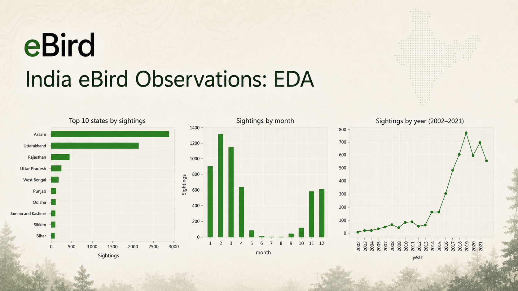
The dataset was obtained the GBIF website and it includes all eBird records for India from 1800 to 2021. It contains roughly 30 millioin rows and takes roughly 3GB disk space.

Memory Footprint Reduction

When loaded with Pandas defaults, the dataframe ate over 2GB of RAM, which is too much to explore comfortably. The fix was simply choosing the right dtype for each column: 32-bit floats for coordinates and counts, small integers for day and month, and categoricals for the repeated string columns like state and species. That alone brought the footprint down to just over 770MB.

def set_dtypes(df):
    df['individualCount'] = df['individualCount'].astype('float32')
    df['decimalLatitude'] = df['decimalLatitude'].astype('float32')
    df['decimalLongitude'] = df['decimalLongitude'].astype('float32')
    df['day'] = df['day'].astype('int8')
    df['month'] = df['month'].astype('int8')
    df['year'] = df['year'].astype('int16')
    df['stateProvince'] = df['stateProvince'].astype('category')
    df['species'] = df['species'].astype('category')
    return df

Trend Analysis for Threatened Species

The goal of this project was to analyze data on endangered species and extract meaningful insights. For that, I focussed on one of my favorite endangered birds in the IUCN Endangered Category: Pallas’s Fish Eagle.

State-wise Counts

My first step was to analyze state-wise counts for the Eagle. I accomplished this using the following code:

state_wise = df_spc.groupby('stateProvince')['individualCount'].sum()
state_wise = state_wise.loc[state_wise != 0].sort_values(ascending=False)
state_wise[:10].plot(kind='bar',title="Top 10 states by sightings")
plt.ylabel("Sightings")
plt.xticks(rotation=90)
plt.show()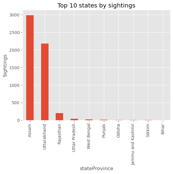

Assam has the highest number of Pallas’ Fish Eagle sightings, with Uttarakhand following closely behind. Sightings in other states drop off significantly, highlighting that Assam and Uttarakhand are the primary regions where this eagle is most commonly observed.

Month-wise Counts

Now the next step was to plot the month-wise counts for Haliaeetus leucoryphus. I did so using the following code:

month_wise = df_spc.groupby('month')['individualCount'].sum()
month_wise = month_wise.loc[month_wise != 0]
month_wise.plot(kind='bar',title="Sightings by month")
plt.ylabel("Sightings")
plt.xticks(rotation=90)
plt.show()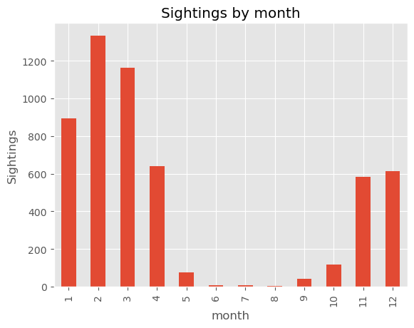

The plot clearly shows an increase in eagle sightings during the winter months, dropping to nearly zero in summer. This pattern confirms that the eagle is indeed a winter visitor to India.

Locality-wise Counts for Assam

Next, I wanted to find out which place/locality in Assam had the highest sightings for the Eagle. That was done using the following code:

top_state = df_spc.query('stateProvince == "Assam"') \
             .groupby(df_spc['locality'])['individualCount'] \
             .sum()
top_state.sort_values(ascending=False)[:20].plot(kind="bar",title="Sightings for Assam")
plt.ylabel("Sightings")
plt.xticks(rotation=90)
plt.show()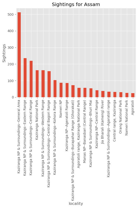

Kaziranga, Manas and Nameri National Parks have many ranges and the records for all of them are present in the data as separate localities, so I had to merge them all.

merged_state = df_spc.query('stateProvince == "Assam"') \
             .groupby(df_spc['locality']\
             .apply(lambda x: re.sub('.*kaziranga.*', 'Kaziranga NP', x, flags=re.IGNORECASE))\
             .apply(lambda x: re.sub('.*nameri.*', 'Nameri NP', x, flags=re.IGNORECASE))\
             .apply(lambda x: re.sub('.*manas.*', 'Manas NP', x, flags=re.IGNORECASE)))['individualCount'] \
             .sum()
merged_state.sort_values(ascending=False)[:15].plot(kind="bar",title="Sightings for Assam")
plt.ylabel("Sightings")
plt.xticks(rotation=90)
plt.show()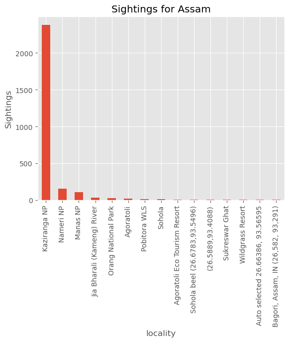

Nearly all sightings of the eagle in Assam come from the various ranges within Kaziranga National Park, while reports from other areas in the state are significantly fewer. This suggests that the national park provides an especially favorable environment and suitable habitat for the species.

Year-wise Trend

Next, I wanted to analyze yearly trends of the Eagle’s sightings. I quickly plotted that using:

yearly = df_spc.groupby('year')['individualCount'].sum()
years = yearly.index.tolist()[-20:]
yearly[-20:].plot(kind="line")
plt.xticks(years,rotation=90)
plt.show()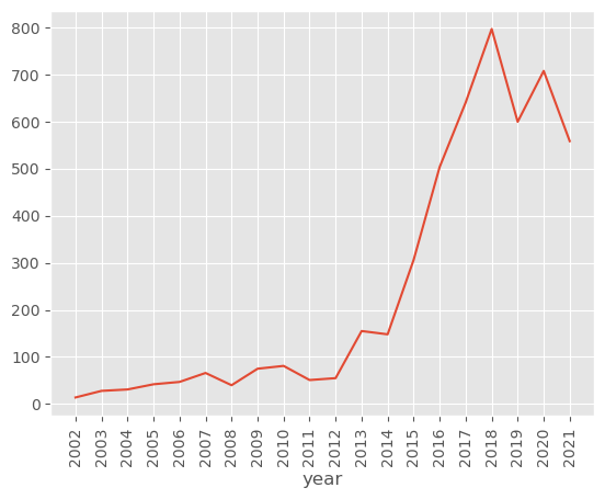

The graph shows a steady increase in eagle sightings across India from 2002 to around 2015, followed by a sharp rise peaking in 2018. Although sightings dip slightly in the following years, they remain significantly higher than in the earlier years, suggesting a notable increase in the eagle’s reported presence across the country over time. This trend could reflect improvements in observation efforts or potential changes in the eagle’s range or population.

The observer-effort confound

Plotting total yearly contributions shows minimal eBird contributions before 2014 and a steep climb from 2015 on.

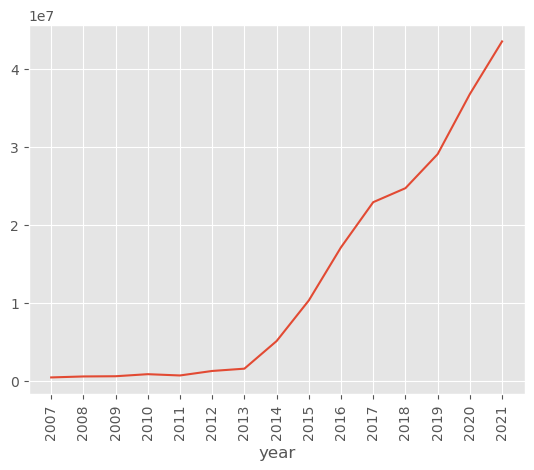
So a rising sighting count does not necessarily mean a rising population, more people are simply looking. Separating real population trends from observer effort is a challenge that I want to explore in further analyses.

On detecting decline

The overall pipeline mostly generalizes to all bird in the dataset, which makes it a useful tool for threatened species. I also tried to automatically flag species in decline, and that turned out to be statistically thorny. Raw percentage change didn’t work as expected on vagrants and species with too few sightings to be significant. Linear regression and the Mann-Kendall test were better but still flagged several vagrants. Despite these challenges, the process was insightful, and refining these methods could lead to more reliable indicators for tracking species trends in the future.